Every time we train a model we should check if its performance beats some baseline, which is a trivial model that doesn’t take the inputs into account. Comparing our model with a baseline model, we can actually figure out whether it actually learns or not.
What is a baseline model?
A baseline model is a model that actually doesn’t use the features, but uses a trivial, constant value for all the predictions. For a regression problem, such a value is often the mean value of the target variable in the training dataset (10 years ago, I used to perform ANOVA tests to compare a linear model with such a trivial model, which was called a null model). For classification tasks, a trivial model just returns the most frequent class in the training dataset.
So, this is the baseline of our dataset and a properly trained model is supposed to beat the performance of such an algorithm. In fact, if a model performs like a baseline, it actually doesn’t consider the features, so it’s not learning. Remember that the given definitions of the baseline models don’t use the features at all, they just average the target values in some way.
In this article, we’re going to see how to compare a model with a baseline model.
The strategy
The general idea is to calculate some performance metrics on the test dataset with both the model and the baseline model. Then, using bootstrap, we calculate the 95% confidence interval of such a measure. If the intervals do not overlap, the model is different from the baseline model.
Doing this procedure, we allow up to 5% probability that the models are actually comparable, in terms of the performance metric we have chosen. Just looking at the mean value of the metric is not enough, unfortunately. Small datasets could introduce finite-size effects that can make our analysis unreliable. That’s why I prefer using bootstrap to calculate the confidence interval, which gives us a better understanding of the situation, extracting as much information as possible from our dataset.
An example in Python
In Python, the baseline model is represented by the DummyClassifier and the DummyRegressor objects. The former considers the most frequent target class in the training dataset, the latter the average value of the target variable. These settings can be changed (for example, by considering the median value in place of the mean value), but I generally prefer to use the default settings because they are pretty realistic and useful.
For a regression problem, we’re going to use “diabetes” dataset and a random forest classifier. Our performance metric will be the r-squared score.
Let’s import some libraries first:
import numpy as np
from sklearn.ensemble import RandomForestClassifier,RandomForestRegressor
from sklearn.model_selection import train_test_split
from sklearn.datasets import load_wine, load_diabetes
from sklearn.dummy import DummyClassifier,DummyRegressor
from sklearn.metrics import accuracy_score, r2_score
Then, let’s import our dataset:
X,y = load_diabetes(return_X_y = True)
X_train,X_test,y_train,y_test  = train_test_split(X,y,test_size=0.4,random_state=0)
We can now train the random forest and the dummy regressor.
model = RandomForestRegressor(random_state=0)
model.fit(X_train,y_train)

dummy = DummyRegressor()
dummy.fit(X_train,y_train)
Finally, with a 500-iteration bootstrap, we can calculate the confidence intervals of the r-squared of our models according to the same test dataset.
scores_model = []
scores_dummy = []
for n in range(500):
  random_indices = np.random.choice(range(len(X_test)),size=len(X_test),replace=True)
  X_test_new = X_test[random_indices]
  y_test_new = y_test[random_indices]

  scores_model.append(r2_score(y_test_new,model.predict(X_test_new)))
  scores_dummy.append(r2_score(y_test_new,dummy.predict(X_test_new)))
Finally, these are the confidence intervals for the model and the dummy classifier:
np.quantile(scores_model,[0.025,0.975]),np.quantile(scores_dummy,[0.025,0.975])
# (array([0.20883809, 0.48690673]), array([-3.03842778e-02, -7.59378357e-06]))
As we can see, the intervals are disjoint and the lower bound of the interval related to the model is greater than the upper bound of the interval related to the dummy model. So, we can say that our model performs better than the baseline with a 95% confidence.
The same approach can be followed using a classifier. The dataset will be the “wine” dataset, for this example. The scoring metric will be the accuracy score.
X,y = load_wine(return_X_y = True)
X_train,X_test,y_train,y_test  = train_test_split(X,y,test_size=0.4,random_state=0)
Here are the models:
model = RandomForestClassifier(random_state=0)
dummy = DummyClassifier()

model.fit(X_train,y_train)
dummy.fit(X_train,y_train)
And here’s the bootstrap for the accuracy score of both models:
scores_model = []
scores_dummy = []
for n in range(500):
  random_indices = np.random.choice(range(len(X_test)),size=len(X_test),replace=True)
  X_test_new = X_test[random_indices]
  y_test_new = y_test[random_indices]

  scores_model.append(accuracy_score(y_test_new,model.predict(X_test_new)))
  scores_dummy.append(accuracy_score(y_test_new,dummy.predict(X_test_new)))
Finally, these are the confidence intervals:
np.quantile(scores_model,[0.025,0.975]),np.quantile(scores_dummy,[0.025,0.975])
# (array([0.91666667, 1.        ]), array([0.31215278, 0.54166667]))
Again, the model performs better than the dummy model with a 95% confidence.
Conclusions
In this article, I show a technique to assess the performance of a model against a trivial, baseline model. Although it’s often neglected, such a comparison is pretty easy to perform and must always be carried out in order to assess the robustness of our model and its generalization capability.


