
Model explanation is an essential task in supervised machine learning. Explaining how a model can represent the information is crucial to understanding the dynamics that rule our data. Let’s see some models that are easy to interpret.
Why do we need to interpret our models?
Data Scientists have the role to extract information from raw data. They aren’t engineers, nor they are software developers. They dig inside data and extract the gold from the mine.
Knowing what a model does and how it works is part of this job. Black-boxes models, although sometimes work better than other models, aren’t a good idea if we need to learn something from our data. On the contrary, some models that are, by their nature, pretty good at explaining how they convert data into information, must always be preferred and deeply studied.
Machine learning models are a way to translate the information into a suitable and understandable language, which is math. If we can translate something into math, we can learn more from it, because we can master math as much as we need. So, a model is not only an algorithm we can write to predict whether a customer will buy something or not. It’s a way to understand “why” a customer with a particular profile would probably buy something and another customer, with a different profile, is not going to buy anything.
So, model interpretation is crucial to give the proper shape to the information we’re looking for.
Interpretation via feature importance
One possible way to interpret how a model “thinks” about our data to extract information is to look at the importance of the features. Importance is usually a positive number. The higher this number, the higher the importance that the model provides to that particular feature.
In this article, I’ll show some models that give us their own interpretation of feature importance using Python and scikit-learn library. Let’s always remember that different models give us different importance to the features. That’s completely normal because each model is a way to look at that wonderful, complex prism that is information. We never have the complete view, so feature importance strongly depends on the model we choose.
Let’s first import some libraries and the “wine” dataset of scikit-learn.
import numpy as np
from sklearn.datasets import load_wine,load_diabetes
from sklearn.tree import DecisionTreeClassifier
from sklearn.ensemble import RandomForestClassifier,GradientBoostingClassifier
from sklearn.linear_model import *
from sklearn.svm import LinearSVC,LinearSVR
import xgboost as xgb
import matplotlib.pyplot as plt
from sklearn.pipeline import make_pipeline
from sklearn.preprocessing import StandardScaler
Let’s now load our dataset and store the names of the features.
X,y = load_wine(return_X_y=True)
features = load_wine()['feature_names']
Now, we are ready to calculate feature importance for different types of models.
Decision trees
Tree-based models calculate the importance of a feature according to the total improvement in the purity of the leaves that it provides across the entire tree. If a feature is able to split a dataset properly and increase the purity of the features, it is important for sure. For simplicity, importance scores in tree-based models are normalized so that they sum up to 1.
In scikit-learn, every decision tree-based model has a property called feature_importances_ which contains the importance of the features. It can be accessed after fitting our model.
Let’s see what happens with a simple decision tree model.
tree = DecisionTreeClassifier()
tree.fit(X,y)

plt.barh(features,tree.feature_importances_)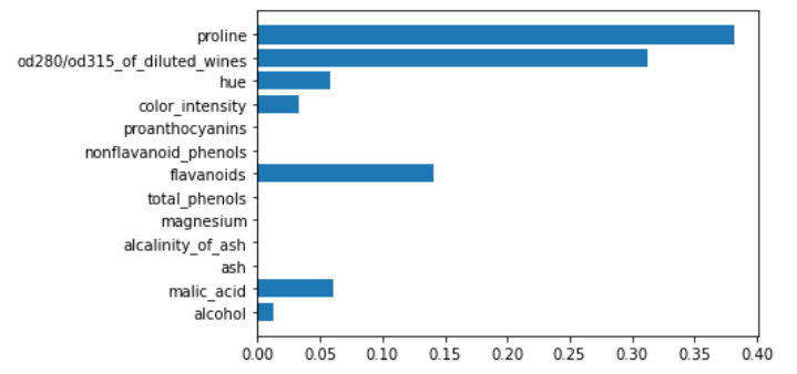
As we can see, some features have importance equal to 0. Maybe they don’t improve purity better than, for example, “proline” feature.
A very important model based on trees that is very useful for feature importance is the random forest. Generally speaking, ensemble models average the importance scores for each feature given by every weak learner and then the final scores are normalized again like in decision trees.
Here’s how to calculate feature importance for a random forest model.
rf = RandomForestClassifier()
rf.fit(X,y)

plt.barh(features,rf.feature_importances_)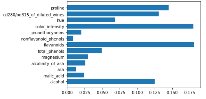
Feature importance given by a random forest can be used to perform feature selection, for example.
Even Gradient Boosting Decision Tree model can give us its own interpretation of feature importance.
gb = GradientBoostingClassifier()
gb.fit(X,y)

plt.barh(features,gb.feature_importances_)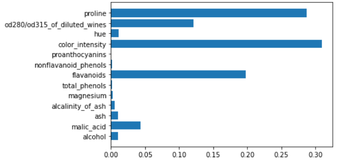
This is true even for XGBoost.
xgboost = xgb.XGBClassifier()
xgboost.fit(X,y)

plt.barh(features,xgboost.feature_importances_)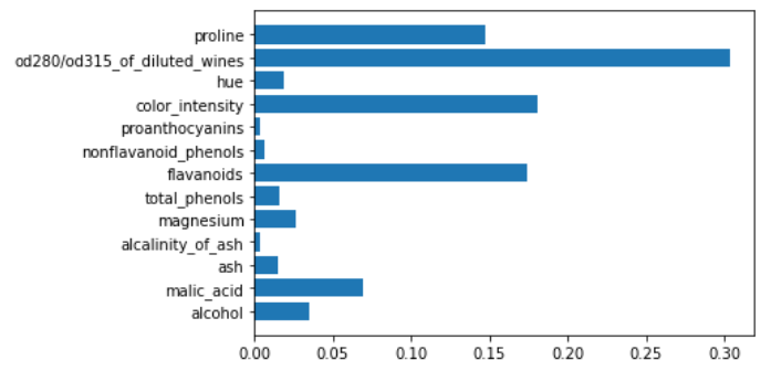
Linear models
Linear models are able to give us feature importance too. It is, actually, the absolute value of the coefficient of a feature. If we work with multi-class linear models for classification, we’ll sum the absolute values of the coefficients related to a single feature.
All the linear models require standardized or normalized features when it comes to calculating feature importance. Several models require this transformation by default, but we always have to apply it if we want to compare the coefficients with each other. That’s why I’ll use the pipeline object in scikit-learn to standardize our data before training the model.
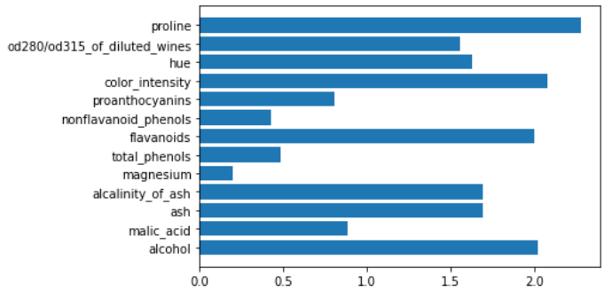
Let’s see an example with the Support Vector Machines with linear kernel.
svm = make_pipeline(StandardScaler(),LinearSVC())

svm.fit(X,y)

plt.barh(features,np.abs(svm[1].coef_).sum(axis=0))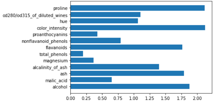
The same applies to logistic regression.
logit = make_pipeline(StandardScaler(),LogisticRegression())

logit.fit(X,y)

plt.barh(features,np.abs(logit[1].coef_).sum(axis=0))
The other linear models that can be used for feature importance are regression models, so we have to load a regression dataset to see how they work. For the following examples, I’ll use the “diabetes” dataset.
X,y = load_diabetes(return_X_y=True)
features = load_diabetes()['feature_names']
Let’s see how linear regression works for calculating feature importance.
lr = make_pipeline(StandardScaler(),LinearRegression())

lr.fit(X,y)

plt.barh(features,np.abs(lr[1].coef_))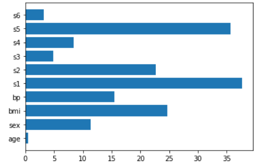
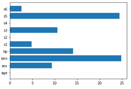
A very powerful model that can be used for feature importance (and for feature selection too) is the Lasso regression
lasso = make_pipeline(StandardScaler(),Lasso())

lasso.fit(X,y)

plt.barh(features,np.abs(lasso[1].coef_))
.
The closest friend to Lasso regression is Ridge regression, which is helpful as well.
ridge = make_pipeline(StandardScaler(),Ridge())

ridge.fit(X,y)

plt.barh(features,np.abs(ridge[1].coef_))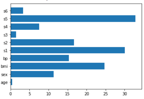
The last model we’re going to see mixes Lasso and Ridge regression together and it’s the Elastic Net regression.
en = make_pipeline(StandardScaler(),ElasticNet())

en.fit(X,y)

plt.barh(features,np.abs(en[1].coef_))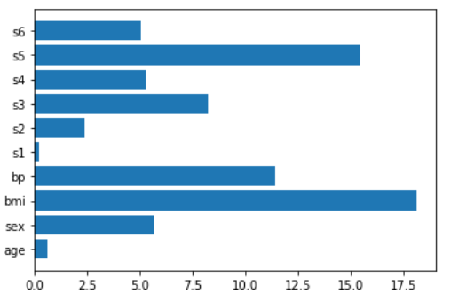
Conclusions
Model interpretation is often done by calculating feature importance and some models give us their own interpretation of the importance of the features. For those models that aren’t able to give feature importance, we can use some model-agnostic approaches like SHAP (very useful to explain neural networks, for example). Proper use of feature importance can improve the value of a Data Science project better than the predictive power of the model itself.