An introduction to linear models

Linear models are some of the simplest models in machine learning. They are very powerful and, sometimes, they are really able to avoid overfitting and give us nice information about feature importance.

Let’s see how they work.

Basic concepts of linear models

All regression linear models share the concept to model the target variable as a linear combination of the input features.

y_{pred} = a_0 + a_1 x_1 + \ldots +a_n x_n

The a_i coefficients are estimated minimizing some cost function.

Linear combination is very simple and is a very common model in nature. Starting from this approach, we can build several different models.

Linear regression

When you have to face a regression problem, Linear regression is always the first choice. This linear model estimates the coefficients minimizing the Mean Squared Error cost function.

\sum_{i = 1}^{N_{training}} \left(y_{real}^{(i)}-y_{pred}^{(i)}\right)^2

This cost function is very simple and the solution of the optimization problem can even be found analytically (although numerical approximations are preferred).

The great problem of linear regression is that it’s sensitive to collinearity, that is the correlation between the features. In fact, if we consider the variance of the prediction, we get:

\sigma_{y_{pred}}^2 = \sum_i a_i^2 \sigma^2_i + \sum_{i \neq j} a_i a_j \rho_{ij} \sigma_i \sigma_j

σ_i is the standard deviation of the i-th feature, while ρ_ij is Pearson’s correlation coefficient between feature i and feature j. It’s clear to see that features with positive correlation increase the prediction variance and this is the greatest issue of linear regression.

In order to avoid collinearity, it’s useful to apply a proper feature selection in advance, taking a look at our dataset during, for example, an Exploratory Data Analysis. Alternatively, Principal Component Analysis can be performed in order to get uncorrelated features.

Ridge regression

Ridge regression modifies the cost function introducing an l₂ penalty term

\sum_{i = 1}^{N_{training}} \left(y_{real}^{(i)}-y_{pred}^{(i)}\right)^2 + \alpha \sum_{j = 1}^n a_j^2

Where α is a hyperparameter. The idea behind Ridge regression is to shrink the values of the coefficients in order to switch useless features off. If α is 0, we return to the original linear regression. If α is too large, we neglect the first part of the cost function and the results are unreliable. So, there’s the need to tune this hyperparameter in order to make the model work properly.

Since we have only one value of α, we need to scale the features in advance. We could use, for example, a standardization technique or other kinds of scaling I talk about in my online course Data pre-processing for machine learning in Python.

Using a penalty function reduces the risk of overfitting, keeping a simple cost function that can be optimized without particular computational effort. In particular situations, Ridge regression may put a feature’s coefficient to 0, applying a sort of automatic feature selection, although Ridge regression is not the best model for such an approach.

Lasso regression

Lasso regression is very similar to Ridge regression, but it uses an l₁ penalty.

\frac{1}{2 N_{training}} \sum_{i = 1}^{N_{training}} \left(y_{real}^{(i)}-y_{pred}^{(i)}\right)^2 + \alpha \sum_{j = 1}^n |a_j|

The great advantage of Lasso regression is that it performs a powerful, automatic feature selection. If two features are linearly correlated, their simultaneous presence will increase the value of the cost function, so Lasso regression will try to shrink the coefficient of the less important feature to 0, in order to select the best features.

Again, like Ridge regression, we need to scale the features in advance in order to make them comparable.

Elastic Net regression

Elastic Net regression mixes Ridge and Lasso together. There is α hyperparameter that tunes the intensity of the penalty part of the cost function, but we have another hyperparameter that is r, which tunes the intensity of l₁ penalty.

The cost function then becomes:

\frac{1}{2 N_{training}} \sum_{i = 1}^{N_{training}} \left(y_{real}^{(i)}-y_{pred}^{(i)}\right)^2 + \alpha r \sum_{j = 1}^n |a_j| + \frac{1}{2} \alpha (1-r) \sum_{j = 1}^n a_j^2

If r is equal to 1, the model becomes a Lasso regression, while if it’s equal to 0 we get a Ridge regression. Intermediate values will mix both models together.

This model mixes advantages and disadvantages of Ridge and Lasso regressions, at the cost of the need to tune 2 hyperparameters. Again, we suffer from collinearity, but the risk of overfitting is pretty low if we tune the hyperparameters correctly.

Logistic regression

Logistic regression is a classification model. It is defined as:

\mathrm{Logistic}(y) = \frac{1}{1+e^{-y}}

where y is

y = a_0 + a_1 x_1 + \ldots +a_n x_n

That’s why logistic regression is considered a linear model.

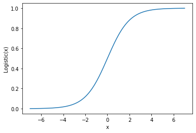
The shape of the logistic function is called sigmoid:

Logistic regression can be used both for binary classification problems and for multi-class classification problems. In the latter case, we just need to one-hot encode the target variable and train a logistic regression on every dummy variable.

When it comes to talking about classification, logistic regression is always the first choice. It’s a very simple model and it works pretty fine, although it may not catch the correct information behind data if the features and the target variable are not linearly correlated.

Again, like any linear model, logistic regression suffers from collinearity and it needs scaled features, in order to avoid the vanishing gradient problem.

Conclusions

Linear models are very simple and useful to use. Moreover, their training is pretty fast and the results can be surprising. We just have to remember to scale the features for those models that require it and to tune the hyperparameters correctly.

Upcoming webinars

If you are interested in linear models, you can register for one of my upcoming webinars.