Are your training and test sets comparable?

Data scientists usually split a dataset into training and test sets. Their model is trained on the former and then its performance is checked in the latter. But, if these sets are sampled wrongly, model performance may be affected by biases.

Should training and test sets be similar?

From the beginning of my career, everybody used to split a dataset into training and test sets randomly and uniformly. It’s a common and generally accepted approach I generally agree with. However, if the training test is statistically different from the training set, the trained model may be affected by a bias and it may not work properly on unseen data.

Think about the complete dataset as a mix of oranges and apples. If we train our model over oranges and test it on apples, it may not work properly. On the contrary, if we create a training dataset that is a mix of oranges and apples, a model trained on such a dataset will work properly on a test set made of oranges and apples.

So, before training our model, we must make sure that training and test datasets are statistically similar.

How to calculate the statistical similarity

In this article, I’ll show how to calculate the statistical similarity between training and test datasets starting from a univariate approach.

The idea is to calculate, for each feature, the cumulative distribution function. We then compare such a function of a feature in the training dataset with the same function of the same feature on the test dataset.

Let’s see an example starting from the diabetes dataset of sklearn. Let’s import it and split it:

from sklearn.datasets import load_diabetes
from sklearn.model_selection import train_test_split

dataset = load_diabetes(as_frame=True)
X,y = dataset['data'],dataset['target']

X_train, X_test, y_train, y_test = train_test_split(X, y, test_size=0.33, random_state=0)

Let’s now plot the cumulative distribution function of ‘bp’ feature for both training and test datasets using seaborn:

feature_name = 'bp'

df = pd.DataFrame({
    feature_name:np.concatenate((X_train.loc[:,feature_name],X_test.loc[:,feature_name])),
    'set':['training']*X_train.shape[0] + ['test']*X_test.shape[0]
    })
sns.ecdfplot(data=df,x=feature_name,hue='set')

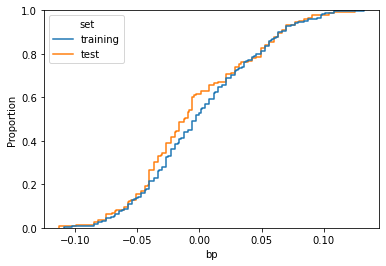
As we can see, the two curves are similar, but there’s a visible difference in the middle. That means that, among the two datasets, the distribution of the feature has been distorted due to the sampling procedure.

In order to quantify the difference between the two distributions with a single number, we can use Kolmogorov-Smirnov distance. Given C(x) the cumulative distribution of feature x in the training dataset and G(x) the cumulative distribution of the same feature in the test dataset, the distance is defined as the maximum distance between these curves.

D_{CG}=\max_x | C(x)-G(x) |

The lower the distance, the more similar the distributions of the features among the training and test datasets.

An easy way to calculate this measure is to use scipy and the K-S test.

The distance is, then:

ks_2samp(X_train.loc[:,feature_name],X_test.loc[:,feature_name]).statistic
# 0.11972417623102555

We can calculate the distance between the two datasets as the maximum distance between their features.

distances = list(map(lambda i : ks_2samp(X_train.iloc[:,i],X_test.iloc[:,i]).statistic,range(X_train.shape[1])))

These are the distances feature by feature:

for i in range(X_train.shape[1]):
  print(X_train.columns[i],distances[i])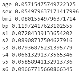

As we can see, the feature that has the lower bias is ‘sex’, while the worst one is ‘bp’. The distance between the datasets is the worst distance, so 0.1197.

If we train and then test a linear model on such datasets using an R-squared score, we get:

lr = LinearRegression()

lr.fit(X_train,y_train)

r2_score(y_test,lr.predict(X_test))

# 0.4033025232246107

How to choose the training and test sets properly

The idea is to generate several couples of training/test datasets and choose the couple that minimizes the distance. The easiest way to create different splits is using the random state.

So, we can loop through several values of the random state, calculate the distance and then select the random state that minimizes it.

Let’s try 100 possible samplings:

n_features = X.shape[1]

n_tries = 100

result = []

for random_state in range(n_tries):
  X_train, X_test, y_train, y_test = train_test_split(X, y, test_size=0.3, random_state=random_state)

  distances = list(map(lambda i : ks_2samp(X_train.iloc[:,i],X_test.iloc[:,i]).statistic,range(n_features)))

  
  result.append((random_state,max(distances)))

result.sort(key = lambda x : x[1])

The resulting distances according to the random states, sorted in ascending order, are:

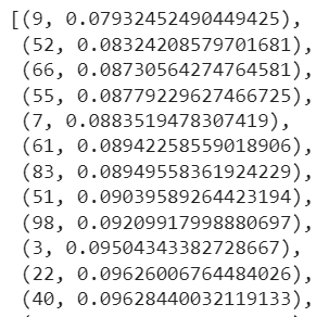
So, the random state that gives us the lowest distance is 9.

Let’s see our ‘bp’ feature on training/test datasets built with this random state.

idx = 0
random_state = result[idx][0]  
feature = 'bp'
X_train, X_test, y_train, y_test = train_test_split(X, y, test_size=0.3, random_state=random_state)

df = pd.DataFrame({
    feature:np.concatenate((X_train.loc[:,feature],X_test.loc[:,feature])),
    'set':['training']*X_train.shape[0] + ['test']*X_test.shape[0]
    })
sns.ecdfplot(data=df,x=feature,hue='set')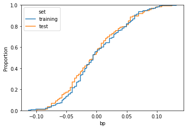

Now the curves overlap much more than before.

The distance is, then:

ks_2samp(X_train.loc[:,feature],X_test.loc[:,feature]).statistic

# 0.07849721390855781

As we can see, it’s lower than the original one.

If we now train the model on these new training and test datasets, the results improve dramatically:

lr = LinearRegression()

lr.fit(X_train,y_train)

r2_score(y_test,lr.predict(X_test))

# 0.5900352656383732

We moved from 40% to 59%. A really strong improvement.

Conclusion

Checking if the training/test split has been correctly performed is crucial when we have to train our models. The procedure suggested in this article is based on Kolmogorov-Smirnov distance and takes into account the features one by one (avoiding the correlation, then). With this simple procedure, you can create datasets that are statistically similar, increasing the training capability of your model.