An example of overfitting and how to avoid it

Overfitting is a tremendous enemy for a data scientist trying to train a supervised model. It will affect performances in a dramatic way and the results can be very dangerous in a production environment.

But what is overfitting exactly? In this article, I explain how to identify and avoid it.

What is overfitting?

Overfitting occurs when your model learns too much from training data and isn’t able to generalize the underlying information. When this happens, the model is able to describe training data very accurately but loses precision on every dataset it has not been trained on. This is completely bad because we want our model to be reasonably good on data that it has never seen before.

Why does it happen?

In machine learning, simplicity is the key. We want to generalize the information obtained from the training dataset, so we can surely say that we run the risk of overfitting if we use complex models.

Complex models will likely over-learn from training data and will think that the random error that drifts training data from the underlying dynamics is actually worth learning from. That’s the exact point at which the model stops generalizing and starts overfitting.

Complexity is often measured with the number of parameters used by your model during it’s learning procedure. For example, the number of parameters in linear regression, the number of neurons in a neural network, and so on.

So, the lower the number of the parameters, the higher the simplicity and, reasonably, the lower the risk of overfitting.

An example of overfitting

Let’s make a simple example with the help of some Python code.

I’m going to create a set of 20 points that follow the formula:

y = -x^2

Each point will be added a normally distributed error with 0 mean and 0.05 standard deviation. In real-life data science, data always drifts from the “real” model by a random error.

Once we have created this dataset, we are going to fit a polynomial model of higher and higher degree and see what happens both in the training set and in the test set. In real life, we don’t know the real model inside our dataset, so we must try different models and see which one fits better.

We’ll take the first 12 points as the training set and the last 8 points as the test set.

First, let’s import some useful libraries:

import numpy as np
import matplotlib.pyplot as plt
from sklearn.metrics import mean_squared_error

Let’s now create the sample points:

np.random.seed(0)
x = np.arange(-1,1,0.1)
y = -x**2 + np.random.normal(0,0.05,len(x))
plt.scatter(x,y)
plt.xlabel("x")
plt.ylabel("y")
plt.show()

As you can see, there’s actually a little noise, just like in real-life fitting.

Now, let’s split this dataset into training and test.

X_train = x[0:12]
y_train = y[0:12]
X_test = x[12:]
y_test = y[12:]

We can now define a simple function that, given the training set and the degree of a polynomial, returns a function that represents the mathematical expression of the polynomial that best fits training data.

def polynomial_fit(degree = 1):
  return np.poly1d(np.polyfit(X_train,y_train,degree))

Let’s now define another function that plots the dataset and the best fitting polynomial with a specific degree.

def plot_polyfit(degree = 1):
  p = polynomial_fit(degree)  plt.scatter(X_train,y_train,label="Training set")
  plt.scatter(X_test,y_test,label="Test set")  curve_x = np.arange(min(x),max(x),0.01)
  plt.plot(curve_x,p(curve_x),label="Polynomial of degree       
      {}".format(degree))  plt.xlim((-1,1))
  plt.ylim((-1,np.max(y)+0.1))
  
  plt.legend()  
  plt.plot()

Now, let’s see what happens with a polynomial of degree 1

plot_polyfit(1)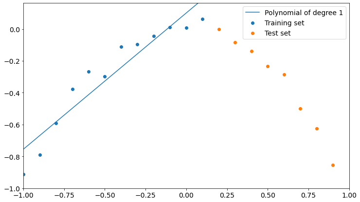

As you can see, a polynomial of degree 1 fits training data better than test data, though it could fit better. We could say that the model is not learning properly from training, so it’s not good.

Let’s see what happens in the opposite case, which is a very high degree polynomial.

Here’s what happens with a polynomial of degree 7.

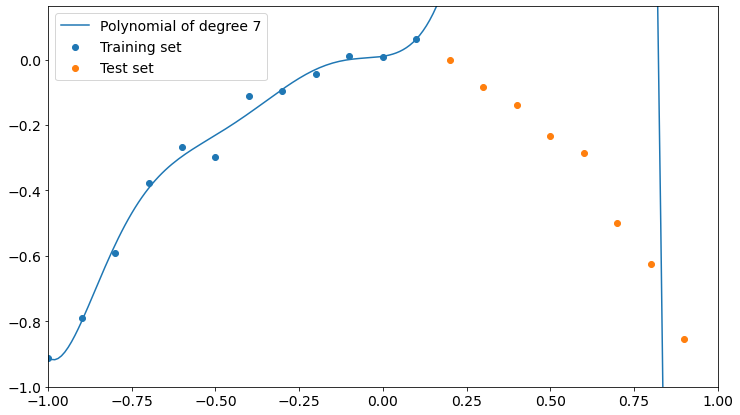
Now the polynomial fits better the training points but it’s completely wrong about the test points.

A higher degree seems to get us closer to overfitting training data and to low accuracy on test data. Remember that the higher the degree of a polynomial, the higher the number of parameters involved in the learning process, so a high-degree polynomial is a more complex model than a low-degree one.

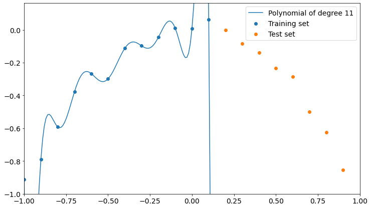
Let’s now see the overfitting explicitly. We have 12 training points and it’s easy to prove that the overfitting can be created with a polynomial of degree 11. It’s called Lagrange polynomial.

Now it’s clear what happens. The polynomial fits training data perfectly but loses precision on the test set. It doesn’t even get close to test points.

So, the higher the degree of the polynomial, the higher the interpolation precision on training data and the lower the performance on test data.

The keyword is “interpolation”. We actually don’t want to interpolate our data, because doing so will make us fit the errors like they were useful data. We don’t want to learn from errors, we want to know the model which is inside errors. That’s why a perfect fit will make a very bad model on unseen data that follow the same dynamics of training data.

How to avoid overfitting

How can we find the right degree of the polynomial? Here comes cross-validation. Since we want our model to perform well on unseen data, we can measure the Root Mean Squared Error of our polynomial with respect to the test data and choose the degree that minimizes this measure.

With this simple code, we loop through all degrees and calculate RMSE for training and test sets.

results = []
for i in range(1,len(X_train)-1):
  p = polynomial_fit(i)
  rmse_training = np.sqrt(mean_squared_error(y_train,p(X_train)))
  rmse_test = np.sqrt(mean_squared_error(y_test,p(X_test)))
  results.append({'degree':i,
    'rmse_training':rmse_training,'rmse_test':rmse_test})

plt.scatter([x['degree'] for x in results],[x['rmse_training'] for x in results],label="RMSE on training")
plt.scatter([x['degree'] for x in results],[x['rmse_test'] for x in results],label="RMSE on test")

plt.yscale("log")
plt.xlabel("Polynomial degree")
plt.ylabel("RMSE")
plt.legend()
plt.show()

Let’s see the results in the following plot:

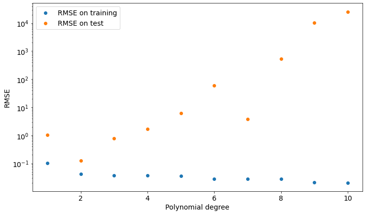
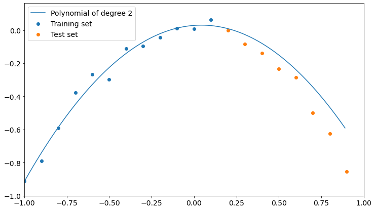
As you can see, we get the lower value of test set RMSE if we choose a polynomial of degree 2, which is the model our data is sampled from.

We can now take a look at such a model and find out that it’s actually pretty good at describing both training and test data.

So, if we want to generalize the underlying phenomena that gave birth to our data, we must cross-validate our model on a dataset it hasn’t been trained on. Only in this way we can be safer about overfitting.

Conclusions

In this simple example, we have seen how overfitting affects model performance and how dangerous it can be if we don’t pay enough attention to cross-validation. Although there are training techniques that are very helpful when it comes to avoiding overfitting (like bagging), we always need to double-check our model in order to make sure it has been trained properly.