
In the machine learning world, data scientists are often told to train a supervised model on a large training dataset and test it on a smaller amount of data. The reason why training dataset is always chosen larger than the test one is that somebody says that the larger the data used for training, the better the model learns.
I’ve always thought that this kind of perspective is actually not completely true and, in this article, I’ll show you why you should keep your training set as small as possible and, instead, reserve the larger part of your data to test purposes.
The problem of measuring model performance
The real task of a supervised model is not learning on the largest dataset possible, but learning in a way that the model performance on unknown data is satisfactory. That’s why we perform the model cross-validation on an unseen dataset.
Data scientists usually provide some model performance metrics calculated on such test datasets, like AuROC, accuracy, precision, root mean squared error and so on. The idea is that if our model performs quite well on unseen data, it will likely perform well in a production environment.
But how accurate is our measure of model’s performance? If I say that my model has an AuROC of 86% on a 100 records test dataset and another person says that another model has still an 86% AuROC but on a 10.000 test dataset, are the two values comparable? Which one would you prefer if you were a manager of a large company and you had been asked to invest some money according to the model prediction?
I’ll give you a spoiler. The larger the test set, the higher the precision of any performance metrics calculated on it.
The precision of model performance
I am a physicist, so I’ve always been told that every measure must be followed by an error estimate. I could tell you I am 1.93 meters tall, but I’m not giving you any information about the precision of this estimate. Is it 1 centimeter, is it 12 centimeters? You can’t tell. The right information could be: I am 1.93 +/- 0.01 m tall, which is 1.93 m with an error estimate of 1 centimeter. If somebody else tries to measure my height, he may obtain 1.93 +/- 0.12 m, which is 1.93 m with an error estimate of 12 centimeters. Which measure is more accurate? Of course the former. Its error is an order of magnitude lower than the latter.
The same approach can be applied to machine learning models. Every time you calculate model performance (e.g. AuROC, accuracy, RMSE), you are performing a measure and this measure must be followed by an error estimate.
So how do you calculate the error estimate on such a measure? There are many techniques, but I prefer using bootstrap, which is a resampling technique that allows you to calculate the standard error and the confidence intervals for an estimate. The standard deviation of the observable among the bootstrap samples is the standard error we can use in our report. It can be easily proofed that the error estimate decreases as the square root of the sample size.
That’s why you must use a large test set. It provides a better estimate of model performance on unseen data.
Example
In the following Python example, I’ll simulate a 1 million records dataset of 4 independent and normally distributed features, then I’ll artificially create a target variable according to the following linear model:
The error between the linear model prediction and the sample y values is normally distributed.
Then I’ll fit the linear model and calculate the RMSE with its standard error and show you that a larger test set gives a smaller standard error, therefore a higher precision for the RMSE value.
You can find the whole code on my GitHub repository.
First, let’s import some libraries.
import numpy as np
from sklearn.model_selection import train_test_split
from sklearn.linear_model import LinearRegression
from sklearn.metrics import mean_squared_error
Let’s simulate 1 million records with 4 normally and independently distributed features.
np.random.seed(0)
X = np.random.normal(size=4000000).reshape(1000000,4)
Now we can create the output variable applying a normally distributed noise.
y = []
for record in X:
   y.append(np.sum(record) + np.random.normal())
   y = np.array(y)
Small test set
Let’s now split our X,y dataset in training and test sets with a test set size that is 20% of the total.
X_train, X_test, y_train, y_test = train_test_split(X, y, test_size=0.2, random_state=42)Now we can fit the linear regression model.
model = LinearRegression()
model.fit(X_train,y_train)
Before calculating model performance, let’s define a function that calculates RMSE and its error estimate with a bootstrapping of 100 samples.
def estimate_error(X_test,y_test):
  n_iter = 100
  np.random.seed(0)
  errors = []  indices = list(range(X_test.shape[0]))
  for i in range(n_iter):
    new_indices = np.random.choice(indices,
        len(indices),replace=True)    new_X_test = X_test[new_indices]
    new_y_test = y_test[new_indices]    new_y_pred = model.predict(new_X_test)    new_error = np.sqrt(mean_squared_error(new_y_test,new_y_pred))    errors.append(new_error)  return np.mean(errors),np.std(errors)
These are the results:
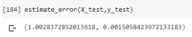
So we have a RMSE equal to 1.0028 +/- 0.0015.
Large test set
What happens if we use a test set that covers 80% of the total population size?
The random split and the model training become:
X_train, X_test, y_train, y_test = train_test_split(X, y, test_size=0.8, random_state=42)model = LinearRegression()
model.fit(X_train,y_train)
The new RMSE estimates are:

So we have 1.00072 +/- 0.00075. Our error has decreased by an order of magnitude, so this last measure is more accurate.
What happened, exactly?
There’s no magic inside these numbers. Simply, it’s an effect of the law of large numbers and of the bootstrapping technique. With larger datasets, any observable estimate in a sample becomes very close to its value on the population it has been drawn from.
Conclusions
Larger test datasets ensure a more accurate calculation of model performance. Training on smaller datasets can be done by sampling techniques such as stratified sampling. It will speed up your training (because you use less data) and make your results more reliable.
References
[1] Gianluca Malato. The bootstrap. The Swiss army knife of any data scientist. Data Science Reporter. https://medium.com/data-science-reporter/the-bootstrap-the-swiss-army-knife-of-any-data-scientist-acd6e592be13
[2] Gianluca Malato. Stratified sampling and how to perform it in R. Towards Data Science. https://towardsdatascience.com/stratified-sampling-and-how-to-perform-it-in-r-8b753efde1ef
[3] Gianluca Malato. How to correctly select a sample from a huge dataset in machine learning. Data Science Reporter. https://medium.com/data-science-reporter/how-to-correctly-select-a-sample-from-a-huge-dataset-in-machine-learning-24327650372c