A Python library to remove collinearity

This post contains affiliate links to products. We may receive a commission for purchases made through these links.

Collinearity is a very common problem in machine learning projects. It is the correlation between the features of a dataset and it can reduce the performance of our models because it increases variance and the number of dimensions. It becomes worst when you have to work with unsupervised models.

In order to solve this problem, I’ve created a Python library that removes the collinear features.

What is collinearity?

Collinearity, often called multicollinearity, is a phenomenon that rises when the features of a dataset show a high correlation with each other. It’s often measured using Pearson’s correlation coefficient. If the correlation matrix shows off-diagonal elements with a high absolute value, we can talk about collinearity.

Collinearity is a very huge problem, because it increases model variance (particularly for linear models), it increases the number of dimensions without increasing the information and, moreover, it distorts our ability to explain a model. If two features are collinear, they shouldn’t be considered together and only the most informative features should be considered.

I’ve been dealing with collinearity for years and finally decided to create a Python library to help other data scientists like me handling this problem efficiently. If you want to know more about collinearity and regression performance, I suggest reading this book.

How to remove collinearity

First, we have to define a threshold for the absolute value for the correlation coefficient. A proper exploratory data analysis can help us identify such a threshold in our dataset, but for a general-purpose project, my suggestion is to use 0.4. It works fine for several types of a correlation although, again, I suggest performing a proper EDA to find the value that fits your dataset.

Once the threshold has been set, we need our correlation matrix to have only off-diagonal elements that are, in absolute value, less than this threshold.

For unsupervised problems, the idea is to calculate the correlation matrix and remove all those features that produce elements that are, in absolute value, greater than this threshold. We can start from the less correlated pair and keep adding features as long as the threshold is respected. This gives us an uncorrelated dataset.

For supervised problems, we can calculate feature importance using, for example, a univariate approach. We can consider the most important feature and then keep adding features following their importance, from the most important one to the less important one, selecting them only if the threshold constraint is respected.

The idea is that adding a feature, we add a new row and a new column in the correlation matrix, so we have to be careful about it. That’s why I’ve created my library.

“collinearity” package

We can easily install my “collinearity” library using pip.

!pip install collinearity

Let’s see it is action in Python.

First, we need to import the SelectNonCollinear object of collinearity package.

from collinearity import SelectNonCollinear

This is the object that performs the selection of the features and implements all the method of sklearn’s objects.

Now, let’s import some useful libraries and the boston dataset.

from sklearn.feature_selection import f_regression
import numpy as np
import pandas as pd
import seaborn as sns
from sklearn.datasets import load_boston
sns.set(rc={'figure.figsize':(12,8)})

Let’s start with the unsupervised approach, in which we don’t know the target variable and just want to reduce the number of the features for clustering problems,

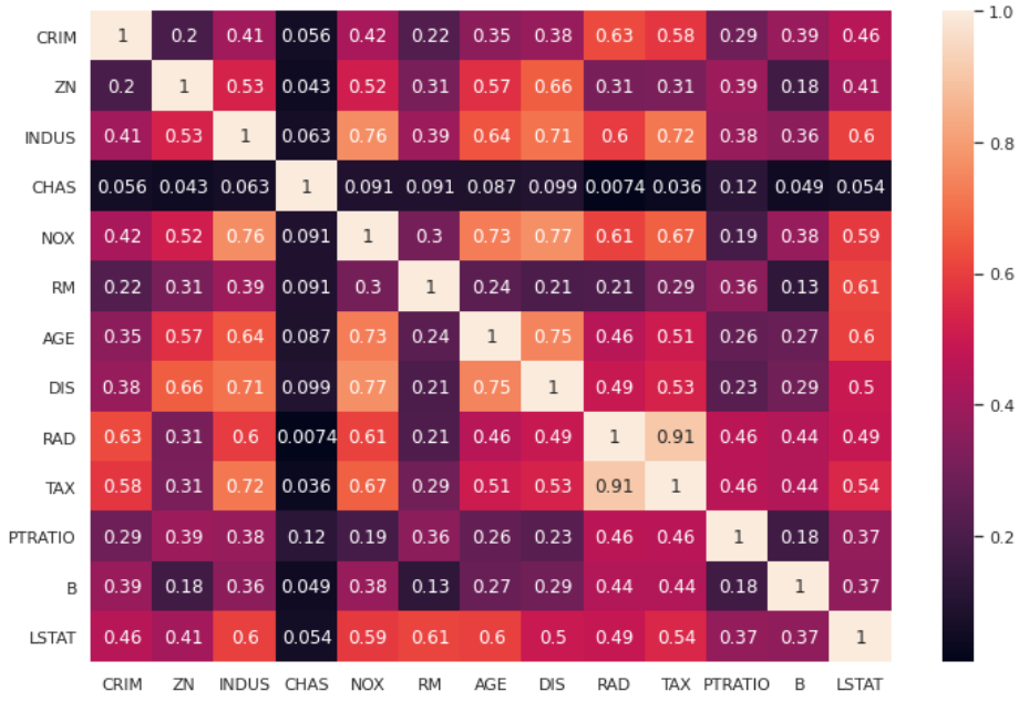
Let’s import our dataset and calculate the correlation heatmap.

X,y = load_boston(return_X_y=True)

features = load_boston()['feature_names']

df = pd.DataFrame(X,columns=features)

sns.heatmap(df.corr().abs(),annot=True)

As we can see, we have several variables that are collinear (i.e. those that have a lighter color in the heatmap)

We can now create an instance of SelectNonCollinear object and set a threshold equal, for example, to 0.4.

selector = SelectNonCollinear(0.4)

As with every scikit-learn object, we have fit, transform and fit_transform methods. We have the get_support method as well, which gives us an array mask for the selected features.

Let’s fit the object and get the mask of the selected features.

selector.fit(X,y)
mask = selector.get_support()

Now we can consider only the selected features and plot the correlation heatmap again:

df2 = pd.DataFrame(X[:,mask],columns = np.array(features)[mask])
sns.heatmap(df2.corr().abs(),annot=True)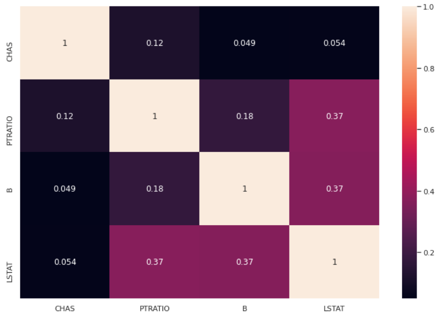

The selected features now show a lower collinearity than the original set and no coefficient is greater than 0.4, as expected.

For the supervised approach, we need to set the scoring function that is used to calculate the importance of a feature with respect to the given target. For regression problems like this one, we can use f_regression. For classification problems we may want to use f_classif.

We need to set this value in the constructor of our instance. Then we can fit our selector again.

selector = SelectNonCollinear(correlation_threshold=0.4,scoring=f_regression)

selector.fit(X,y)
mask = selector.get_support()

We can now calculate the new heatmap, which is, in this example, the same as the unsupervised case.

df3 = pd.DataFrame(X[:,mask],columns = np.array(features)[mask])
sns.heatmap(df3.corr().abs(),annot=True)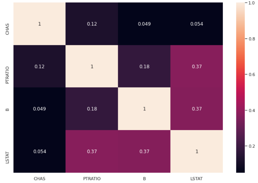

If we just want to filter our dataset, we can easily invoke the transform method.

selector.transform(X)

# array([[  0.  ,  15.3 , 396.9 ,   4.98],
#        [  0.  ,  17.8 , 396.9 ,   9.14],
#        [  0.  ,  17.8 , 392.83,   4.03],
#        ...,
#        [  0.  ,  21.  , 396.9 ,   5.64],
#        [  0.  ,  21.  , 393.45,   6.48],
#        [  0.  ,  21.  , 396.9 ,   7.88]])

This allows us to use SelectNonCollinear object inside an sklearn’s pipeline.

pipeline = make_pipeline(
    SelectNonCollinear(correlation_threshold=0.4,scoring=f_regression),
    LinearRegression()
)

pipeline.fit(X,y)

In this way, we can implement this object inside our ML pipelines effortlessly.

Conclusions

I’ve implemented this library for removing collinearity both for unsupervised and of supervised machine learning projects. The value of the threshold should be set according to a proper EDA. It may happen that, for some datasets like the one used in this example, the selected features are the same between the unsupervised and the supervised approach. My suggestion is to use the correct method according to our problem.

If you have any comments, issues or suggestions, feel free to use my GitHub repo: https://github.com/gianlucamalato/collinearity