
Statistics is a must-have skill in a Data Scientist’s CV, so there are concepts and topics that must be known in advance if somebody wants to work with data and machine learning models.
Probability distributions are a must-have tool. Let’s see the most important ones to know for a Data Scientist.
Uniform distribution
The simplest probability distribution is the uniform distribution, which gives the same probability to any points of a set.
In its continuous form, a uniform distribution between a and b has this density function:
And here’s how it appears.

As you can see, the wider the range, the lower the distribution. This is necessary to keep the area equal to one.
The uniform distribution is everywhere. Any Monte Carlo simulation starts by generating uniformly distributed pseudo-random numbers. The uniform distribution is used, for example, in bootstrapping techniques for calculating confidence intervals. It’s a very simple distribution and you’ll find it very often.
Gaussian distribution
The queen of all distributions and maybe the most known.If you have some random and independent variables with finite variance, the probability distribution of their sum converges towards a Gaussian distribution.
This is the probability density function:
μ and σ are the mean and the standard deviation of the distribution. The mean is the peak position, while the standard deviation is related to the width. The higher the standard deviation, the larger the distribution (and the lower the peak, to keep area equal to 1).
A particular case of gaussian distribution is the normal distribution, whose mean is equal to 0 and the standard deviation is equal to 1.
Every regression model using the least-squares approach assumes that the residuals are normally distributed, so it’s important to know if our data is normally distributed.The F test for comparing variances of the residuals of a model in two datasets assumes that the residuals are normally distributed. If you work with data science, you and the Gaussian distribution will become best friends soon.
Student’s t distribution
A very particular distribution is Student’s t distribution, whose probability density function is:
The free parameter n is called “degrees of freedom” (often abbreviated in d.o.f.). It’s easy to show that t distribution gets closer to a normal distribution for high values of n.

If you have to compare mean values of different samples or the mean value of a sample with the mean value of a population and if the samples are taken from a Gaussian distribution, you’ll often use Student’s t-test, which is a hypothesis test performed using Student’s t distribution. It’s also possible to use Student’s t-test to check the linear correlation between two variables. So it’s very likely that you’ll need this distribution someday in the future in your Data Scientist career.
Chi-squared distribution
If you take some normally distributed and independent random variables, take their square value and sum them, you get a chi-square variable, whose probability density function is:
k is the number of degrees of freedom. It’s often equal to the number of the squared normal variables you sum, but sometimes it’s reduced if there’s some relationship between these variables (for example, the number of model parameters in a curve-fitting problem).
Here are some examples of this distribution.

You’ll use chi-squared distribution in Pearson’s chi-square test, which compares an experimental histogram with a theoretical distributionunder certain assumptions. The chi-squared distribution is related to the F test for the equality of variances because the F distribution is calculated as the probability distribution of the ratio between two chi-square variables.
Lognormal distribution
If you take a gaussian variable and exponentiate it, you get the lognormal distribution, whose probability density function is:
μ and σ are the same as the original gaussian distribution.
Here are some examples:

The lognormal distribution is widely measured in nature. Blood pressure follows a lognormal distribution, city sizes, and so on. A very interesting use is in the geometric Brownian motion, which is a model of random walk often used to describe financial markets, particularly in the Black-Scholes equation for options pricing.
Just like Gaussian distribution is widely present in nature for observables in the real domain, lognormal distribution is almost as frequent for observables with positive values. You can notice a strong asymmetry and a long tail, both very frequent phenomena in many situations when you deal with positive variables.
Binomial distribution
The binomial distribution is often described as the coin toss probability distribution. It measures the probability of two events, one of them occurring with probability p and the other one occurring with probability 1-p.
If our events are 0 and 1 numbers and the 1 event occurs with p probability, we can easily write the density using Dirac’s delta distribution:
A possible representation is as follows:

The binomial distribution is the basic tool for any probability course and, in a Data Scientist’s career, can occur many times. Just think about binary classification models, that work with a 0–1 variable and its statistics.
Poisson distribution
Poisson distribution is often described as the distribution of rare events. Generally speaking, if you have an event that occurs with a fixed rate in time (i.e. 3 events per minute, 5 events per hour), the probability of observing a number n of events in the time unit can be described with Poisson distribution, which has this formula:
μ is the event rate in a time unit.
Here are some examples:
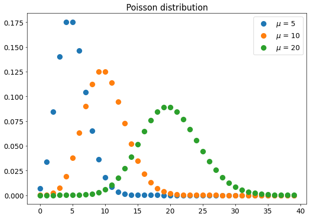
As you can see, its shape is similar to a gaussian distribution and its peak is equal to μ.
Poisson distribution is very used in particle physics and, in data science,it can be useful to describe events that have a fixed rate (e.g. a customer that enters into a supermarket in the morning).
Exponential distribution
If you have a Poisson event that occurs at a fixed time rate, the time interval between two consecutive occurrences of that event is exponentially distributed.
Exponential distribution has this density function:
τ is the average time interval between two consecutive events.
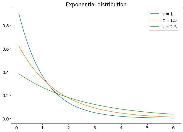
The exponential distribution is used in particle physics and, generally speaking, if you want to move from a Poisson process (in which you study the number of events) to something more related to time (e.g. how much time occurs between two consecutive customers entering into a shop).
Conclusions
Data Science and statistics are two very related topics and it’s not possible to work well with the former if you don’t know the latter. In this article, I’ve shown you some of the most important probability distributions you’ll find during your Data Scientist career. Other distributions (e.g. Gamma distribution) can be found, but it’s likely that in a Data Scientist’s daily job he will work with one of the distributions described here.